Due to the robot moving at rates faster than my TOF sensors can gather data I need implemenet something that can predict potential measurements so that my robot can act accordingly. This lead to the implemenataion of a Kalman filter which can gather potential data at a much faster rate than the TOF sensors.
To fully implement the Kalman Filter I needed to be able to find the drag and momentum of my robot.
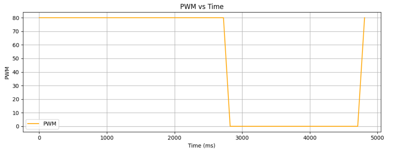
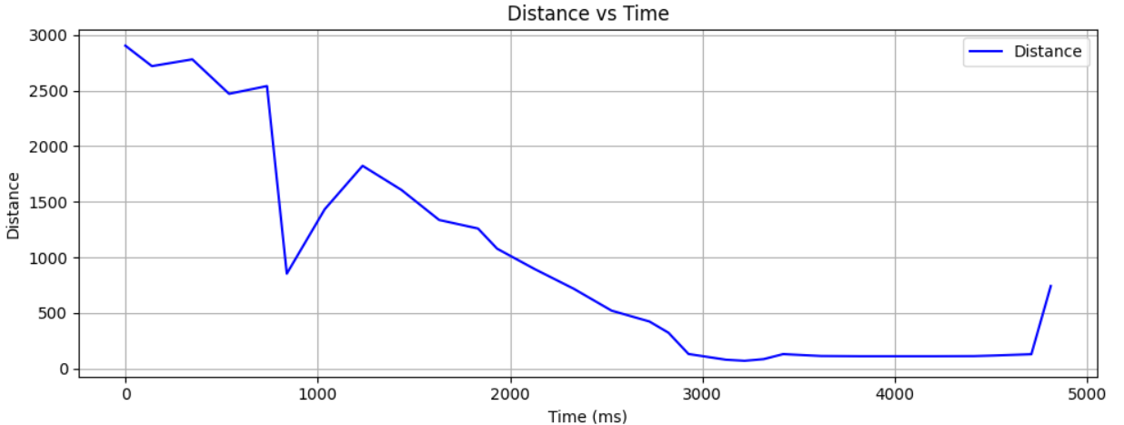
To estimate these two I needed to choose a step response around 50% - 100% of the PWM value I used in Lab 5. Thus I choose the PWM value to be 80 which also was the value used in lecture to explain the filter and the process to create one. I then placed my robot 7 ft away from a wall and sent my robot towards said wall so that it gave my robot ample time to get a steady state velocity that can be helpful to implement the filter. After doing this test I was able to gather these graphs that show the PWM value, TOF distance readings, and Velcoity of the robot:
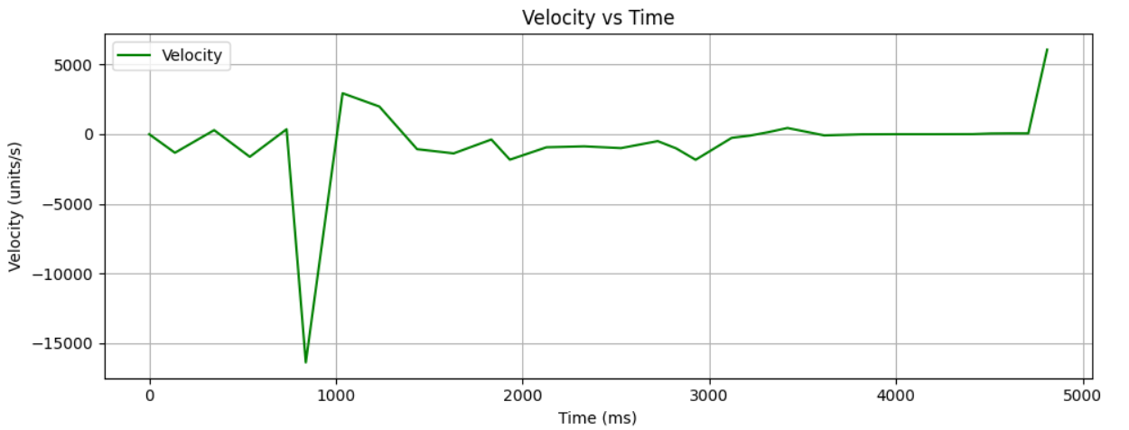
From this I found the steady state portion of my veloctiy graph by running this portion of code:
        # Find indices where PWM == 80 and time > 1000 ms
        steady_indices = [i for i in range(len(time)) if pwm[i] == 80 and time[i] >= 1000]

        # Extract corresponding steady-state velocities
        steady_state_portion = [velocity[i] for i in steady_indices]

        # Compute average steady-state speed
        if steady_state_portion:
            Average_speed = sum(steady_state_portion) / len(steady_state_portion)
            print("Steady-state speed:", Average_speed)
        else:
            print("No steady-state portion found.")
I then used the average_speed from the steady state portion of the velocity graph to find which was 274.94 ms which was around 0.9 seconds. I then throw those values into the drag and momentum formaulas:
            d=1/Average_speed
            m=-0.9/np.log(0.1)
In the end I found that the drag was 0.0036371321381966503 and the momentum was found to be 0.3908650337129267. This then lead me to be able to create my A and B matrcies from lecture:
Since matrix C was already given with values inside of it I was able to find A and B discretize them create a state vector and create noise matrices.
        A = np.array([[0,1],[0,-d/m]])
        B = np.array([[0], [1/m]])  # shape (2,1)
        C = np.array([[-1, 0]])  # 2D row vector shape (1,2)
        dt = time[1] - time[0]
        Ad = np.eye(2) + dt * A
        Bd = dt * B
        x = np.array([[tof2_distance[0]],[0]])
        sig1 = 1
        sig2 = 10
        sig3 = 1
        sig_u = np.array([[sig1** 2, 0],[0,sig2**2]])
        sig_z = np.array([[sig3**2]])
In the end I used the code from lecture to fully implement a Kalman Filter function to gather predicted TOF distance data.
        def kalman_filter(mu,sigma,u,y):
        mu_p = A.dot(mu) + B.dot(u)
        sigma_p = A.dot(sigma.dot(A.transpose())) + sig_u

        sigma_m = C.dot(sigma_p.dot(C.transpose())) + sig_z
        kkf_gain = sigma_p.dot(C.transpose().dot(np.linalg.inv(sigma_m)))

        y_m = y - C.dot(mu_p)
        mu = mu_p + kkf_gain.dot(y_m)
        sigma = (np.eye(2) - kkf_gain.dot(C)).dot(sigma_p)

        return mu,sigma
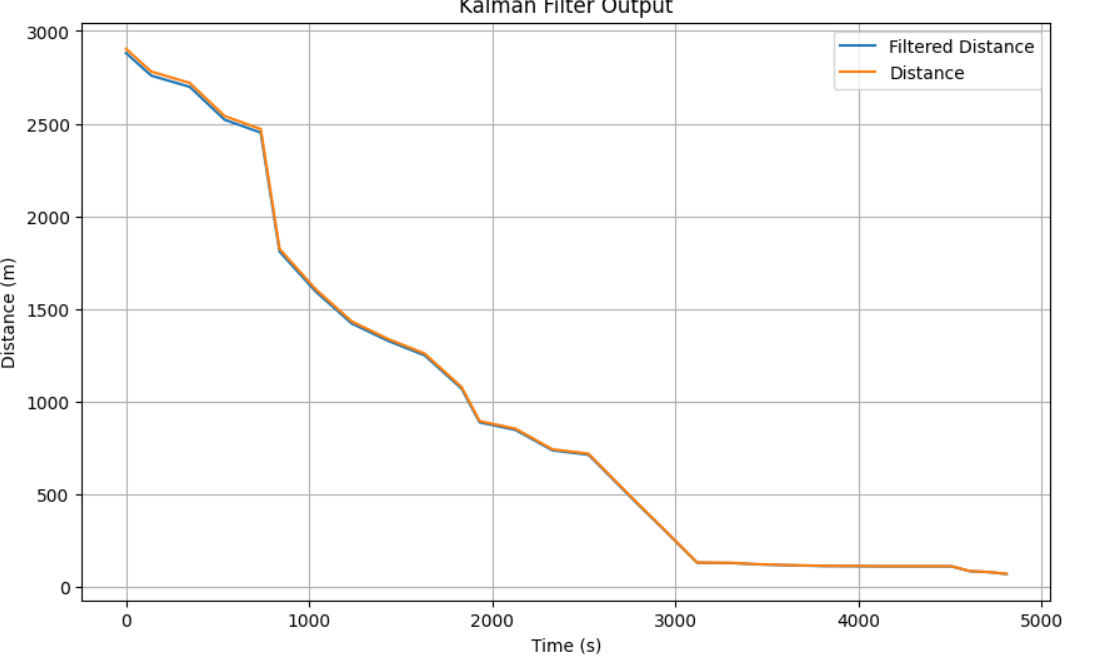
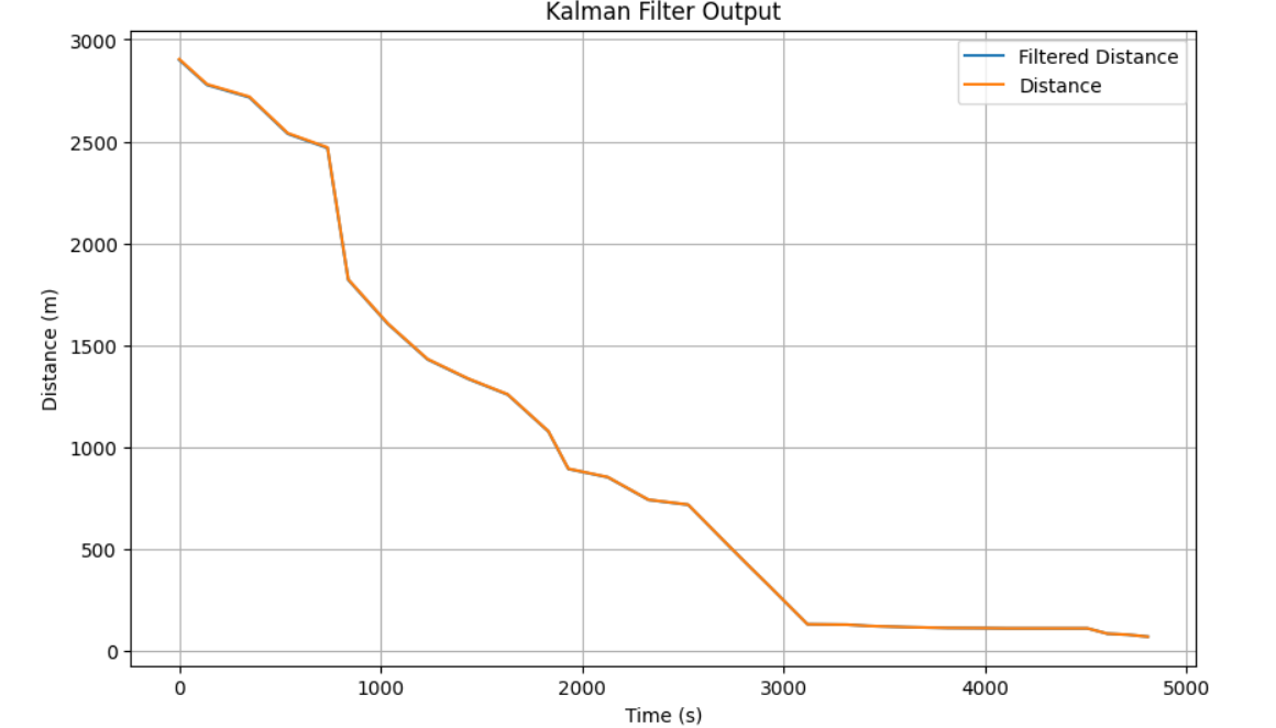
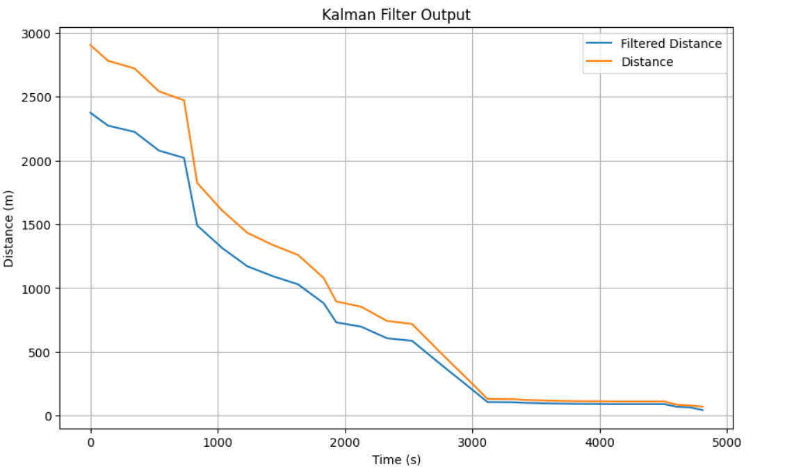
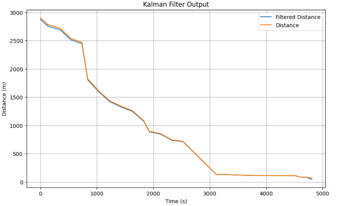
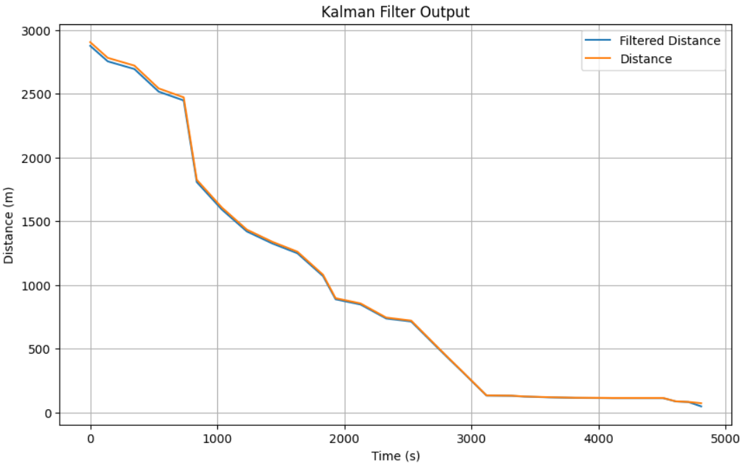
Below is the graphs gathered from testing the Kalman Filter with their respected sigmas.
        sig1 = 40
        sig2 = 40
        sig3 = 5
        sig1 = 20
        sig2 = 20
        sig3 = 1
        sig1 = 30
        sig2 = 30
        sig3 = 20
        sig1 = 20
        sig2 = 1
        sig3 = 1
        sig1 = 1
        sig2 = 10
        sig3 = 1