The primary objective of this lab was to create a 2D map of a static environment (e.g., the lab space, a hallway)
using distance measurements obtained from Time-of-Flight (ToF) sensors mounted on the robot. The robot was programmed
to rotate in place at several known locations, collecting sensor data during the rotation. This data was then processed
using Python and merged to generate a representation of the surrounding obstacles.
Material List
1 x Fully assembled robot, with Artemis, TOF sensors, and an IMU
Approach: Open-Loop Control
For controlling the robot's rotation during scanning, the open-loop timed turn approach was selected. This method involves
running the motors for a predetermined duration at a fixed speed to achieve an approximate angular increment between sensor readings.
While this is the simplest control strategy to implement, it comes with significant drawbacks regarding accuracy.
Implementation Choice: Timed incremental turns were used. The robot turns, stops briefly (implicitly, during the delay between motor commands and sensor reading), reads sensors, and repeats.
Rationale: This approach was chosen primarily due to time contraints. Still at the current moment I have trying to iron out the issues with my PID controler when it comes to the orienation of the robot.
Trade-offs: The main advantage is implementation speed. The major disadvantage is the inherent inaccuracy of the turns. Factors like battery voltage fluctuations, variations in floor friction, and motor inconsistencies directly impact the actual angle turned, leading to non-uniform angular spacing between readings and potential map distortion.
Tuning: The duration `MAP_OPEN_LOOP_TURN_DURATION_MS` in the Arduino code required experimental tuning. The value was set to `350` ms based on visual observation aiming for approximately 20-degree increments per step.
Lab Tasks
Control Implementation (Open Loop)
The open-loop control was implemented within the `MAP_ENVIRON` command case in the Arduino firmware. The core logic involves:
Starting a loop that runs for a maximum number of turns (18) or a time limit.
Inside the loop, activating the motors to turn the robot in place (e.g., one motor forward, one backward) at `MAP_OPEN_LOOP_TURN_SPEED`.
Waiting for a fixed duration using `delay(MAP_OPEN_LOOP_TURN_DURATION_MS)`.
Stopping the motors.
Reading data from the ToF sensors.
Repeating the process.
The relevant Arduino code snippet controlling the turn:
// --- Open-Loop Timed Turn Logic ---
Serial.print("  Turning for "); Serial.print(MAP_OPEN_LOOP_TURN_DURATION_MS); Serial.println(" ms...");
// Activate motors for turning
analogWrite(MotorPin1, 80); // Example: Right motor forward for right turn
analogWrite(MotorPin2, 0);
analogWrite(MotorPin3, 0);  // Example: Left motor backward for right turn
analogWrite(MotorPin4, 100);
// Wait for the specified duration
delay(MAP_OPEN_LOOP_TURN_DURATION_MS);
// Stop motors
analogWrite(MotorPin1, 0);
analogWrite(MotorPin2, 0);
analogWrite(MotorPin3, 0);
analogWrite(MotorPin4, 0);
Serial.println("  Turn complete (timed).");
// --- End Turn Logic ---
Turn Performance Documentation
Due to the open-loop nature, precise quantification is difficult. Visual inspection suggested turns were roughly 15-20 degrees per step. The robot was able to consisently be an angle closer to 20 degrees but with the error caused by the human eye and the absence of a protractor leasds to a loose conclusion.
Video of Open-Loop Turn:
[Video Placeholder: Embed or link to a video showing the robot performing the timed turns.]
Data Collection
The robot was supposed to be placed at various locations in the my room but due to a last minute battery detachment I could not test the robot past the intial spot it was placed in:
Location 1: (-3, -3)
Location 2: (0,3)
Location 3: (5,-3)
Location 4: (5,3)
At each location, the robot was started facing the same initial direction facing north towards the windows in my room.
The `MAP_ENVIRON` command was initiated via Bluetooth using a Python script. This script connected to the robot, sent the command, and registered a notification handler (`map_handler`) to receive the stream of data strings from the Artemis board's `RX_STRING` characteristic.
The handler parsed the incoming comma-separated strings (containing Timestamp, Distance1, Distance2, Intended Total Angle) and stored the values in Python lists.
Example Python code snippet for receiving data:
# Placeholder lists
time=[]
dist1=[]
dist2=[]
angle= [] # Stores the 'Intended Total Angle' received from Arduino

# BLE Notification Handler
def map_handler(uuid, byte_array):
    global time, dist1, dist2, angle
    try:
        # Decode byte array and split CSV data
        s = ble.bytearray_to_string(byte_array).split(",")
        # Extract values based on expected format from Arduino
        # Assumes format like "T:val,D1:val,D2:val,AngT:val"
        time.append(s[0].split(":")[1])
        dist1.append(s[1].split(":")[1])
        dist2.append(s[2].split(":")[1])
        angle.append(s[3].split(":")[1]) # Captures the intended total angle
        # Note: Original Python code had a 5th element 'acta', adjust if needed
    except Exception as e:
        print(f"Error parsing BLE data: {e} - Received: {ble.bytearray_to_string(byte_array)}")

# Start notifications and send command (inside main script logic)
# ble.start_notify(ble.uuid['RX_STRING'], map_handler)
# ble.send_command(CMD.MAP_ENVIRON, "")
# # Add logic to wait for data collection to finish...
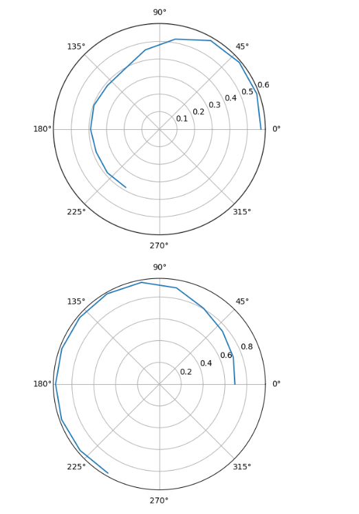
Scan Sanity Check (Polar Plots)
To verify the data from individual scans, polar plots were generated for each location using Matplotlib in the Python script. Since open-loop control was used, the angle for each reading was derived from the *intended total angle* (`AngT`) received from the Arduino. This assumes equal angular spacing, which is likely inaccurate but necessary without reliable orientation feedback.
Example Python code for generating polar plots:
# Assumes 'angle' list contains intended total angles (degrees)
# Assumes 'dist1', 'dist2' lists contain distances (converted to meters)
import numpy as np
import matplotlib.pyplot as plt

# Offset angles to start from 0
a_offset = angle[0] if angle else 0
plot_angles = [a - a_offset for a in angle]

# Plot for Sensor 1
plt.polar(np.radians(plot_angles), dist1, marker='o', linestyle='none')
plt.title('Polar Plot - Sensor 1 - Location [X,Y]')
plt.show()

# Plot for Sensor 2
plt.polar(np.radians(plot_angles), dist2, marker='o', linestyle='none')
plt.title('Polar Plot - Sensor 2 - Location [X,Y]')
plt.show()
Polar Plot - Location 1
This polar plot shows what the robot was able to see in the in one of the marked spots in the map. The reason there is only one plot is becaused the other polar plots looked very similar but had different orientations.
Data Processing & Merging
To combine the data from all locations into a single map relative to the room's origin, coordinate transformations were required. This was implemented in the jupyter notebook script using NumPy.
Transformation Matrices
Two main transformations were needed for each data point:
Sensor Frame to Robot Frame: Converts the distance reading into Cartesian coordinates (x, y) relative to the robot's center. The Python script assumes Sensor 1 points forward along the robot's local x-axis and Sensor 2 points backward (negative x-axis).
(Note: This assumes sensors are at the origin (0,0) of the robot frame. Adjust if sensors have offsets.)
Robot Frame to World Frame: Transforms the point relative to the robot into the global coordinate system using the robot's known world position (X_R, Y_R) and its *intended* orientation (Theta_R) at the time of the reading.
The Python script uses homogeneous coordinates and matrix multiplication to perform the rotation and translation:
import numpy as np

# Example for one location (e.g., data_1 from location x, y)
# acta_1 = np.radians(angle_data_from_location_1) # Intended angles in radians
# dist1_1, dist2_1 = distance_data_from_location_1 # Distances in meters
# x, y = robot_world_position_for_location_1 # e.g., x=-3, y=-2

position1_tof1 = []
position1_tof2 = []

for i in range(len(acta_1)):
    # Sensor reading in robot frame (homogeneous coords)
    # Sensor 1 assumed forward (+x), Sensor 2 assumed backward (-x)
    tof1_robot_h = np.array([[dist1_1[i]], [0], [1]])
    tof2_robot_h = np.array([[-dist2_1[i]], [0], [1]]) # Note the negative sign

    # Transformation matrix: Rotation by intended angle + Translation to world pos
    theta = acta_1[i] # Intended angle for this reading
    r_matrix = np.array([
        [np.cos(theta), -np.sin(theta), x],
        [np.sin(theta),  np.cos(theta), y],
        [0,              0,             1]
    ])

    # Apply transformation
    world_pt_tof1 = np.matmul(r_matrix, tof1_robot_h)
    world_pt_tof2 = np.matmul(r_matrix, tof2_robot_h)

    position1_tof1.append(world_pt_tof1)
    position1_tof2.append(world_pt_tof2)

# Extract x, y coordinates for plotting
tof1_x_world = np.array(position1_tof1)[:, 0, 0]
tof1_y_world = np.array(position1_tof1)[:, 1, 0]
tof2_x_world = np.array(position1_tof2)[:, 0, 0]
tof2_y_world = np.array(position1_tof2)[:, 1, 0]
The sesnors were mounted on the robot by having one TOF sensor at the front of the robot and one TOF sensor at the back of the robot. Also when allowing the robot to turn and spin around the robot was always placed on the floor facing north/parallel to the y axis.
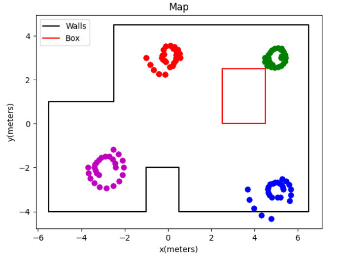
Merged Scatter Plot
After applying the transformations to all valid distance readings from all locations, the resulting world coordinates (x_w, y_w) were plotted together using Matplotlib. Data from each scan location was assigned a different color for clarity, as shown in the final plotting section of the Python script.
Merged Scatter Plot of All ToF Readings
[Comment on the overall appearance.]
Line-Based Map Generation
Based on the merged scatter plot, wall segments and major obstacles were manually estimated and drawn as straight lines. This involved visually interpreting the clusters of points and connecting them logically.
Error Sources
Potential sources of error influencing this step include:
Inaccurate robot orientation (Theta_R) due to open-loop timed turns, causing rotation/misalignment of scans.
Inaccurate robot position (X_R, Y_R) if placement wasn't precise, causing translation offsets.
Sensor noise or erroneous readings (e.g., reflections, readings beyond max range, crosstalk).
Simplifications in the Sensor-to-Robot frame transformation (e.g., assuming sensors are exactly at the origin).
Due to the friciton of the floor mixed with the intial volatge needing to be sent to the robot to make it move I noticed that not every turn was not 20 degrees but was close. This caused me to sometimes move the robot so that was more accurately a 20 degree turn. Also I noticed that when placing the robot closer to the marked positions the robot struggled more to turn so I placed the robot within the same tile as the marked location but not directly above the tape on the floor.
Final Map
Final Line-Based Map
Map Data (Line Endpoints)
The endpoints of the line segments representing the map obstacles are:
# List of starting points (x_start, y_start) in meters
map_starts = [
    (x1_start, y1_start),
    (x2_start, y2_start),
    # ... add all starting points
]

# List of ending points (x_end, y_end) corresponding to starts in meters
map_ends = [
    (x1_end, y1_end),
    (x2_end, y2_end),
    # ... add all ending points
]
Shown below is the plots at each point of the map.:
Conclusion
This lab successfully demonstrated the process of creating a 2D map using ToF sensors and an open-loop rotation strategy, with data processing performed in Python. While the open-loop approach allowed for rapid implementation, the resulting map's accuracy, visualized through the Python-generated plots, was clearly limited by the inconsistencies in the timed turns. The transformation process implemented in Python highlighted the importance of accurate robot pose (position and orientation) estimation for merging sensor data correctly.
 This polar plot shows what the robot was able to see in the in one of the marked spots in the map. The reason there is only one plot is becaused the other polar plots looked very similar but had different orientations.
 [Comment on the overall appearance.]
.png)
.png)
.png)
.png)